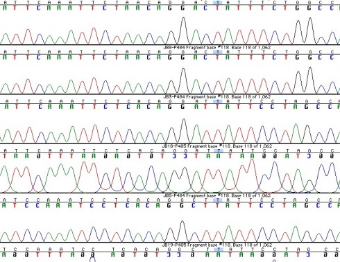
In early October we received our sequence data back from the Yale DNA Analysis Facility. The sequence data gave us both the forward and reverse strands that we copied using PCR for each of our rodent species. We had two samples with either shortened or ruined sequence data for one strand that we could not use, but even so we had one sequence with a decent enough result that we could read the whole length from the one strand that worked. The next step that we took was to pull the sequence data up in a sequence editing program and arrange the sequences into “contigs”; this means we paired the sequences into groups of forward and reverse strands so that we could edit the sequences. We have to edit the sequences because the machine can make mistakes and make the wrong call on certain bases where it has overlapping base signals or weak data. We edited the sequences by first comparing the forward and reverse strands for individual samples to see if the strands matched; the purpose for having both strands is so that there will be overlap that can be used for comparison. Sequence data is often weaker and less reliable farther down the strand from its given primer so having the other side allows for clearer data at the extreme ends. As we got farther into the editing we compared larger groups of samples together so that we could see the similarities and make sure we made consistent ‘calls’ during the editing process.

DNA Data in a Sequence Editing Program
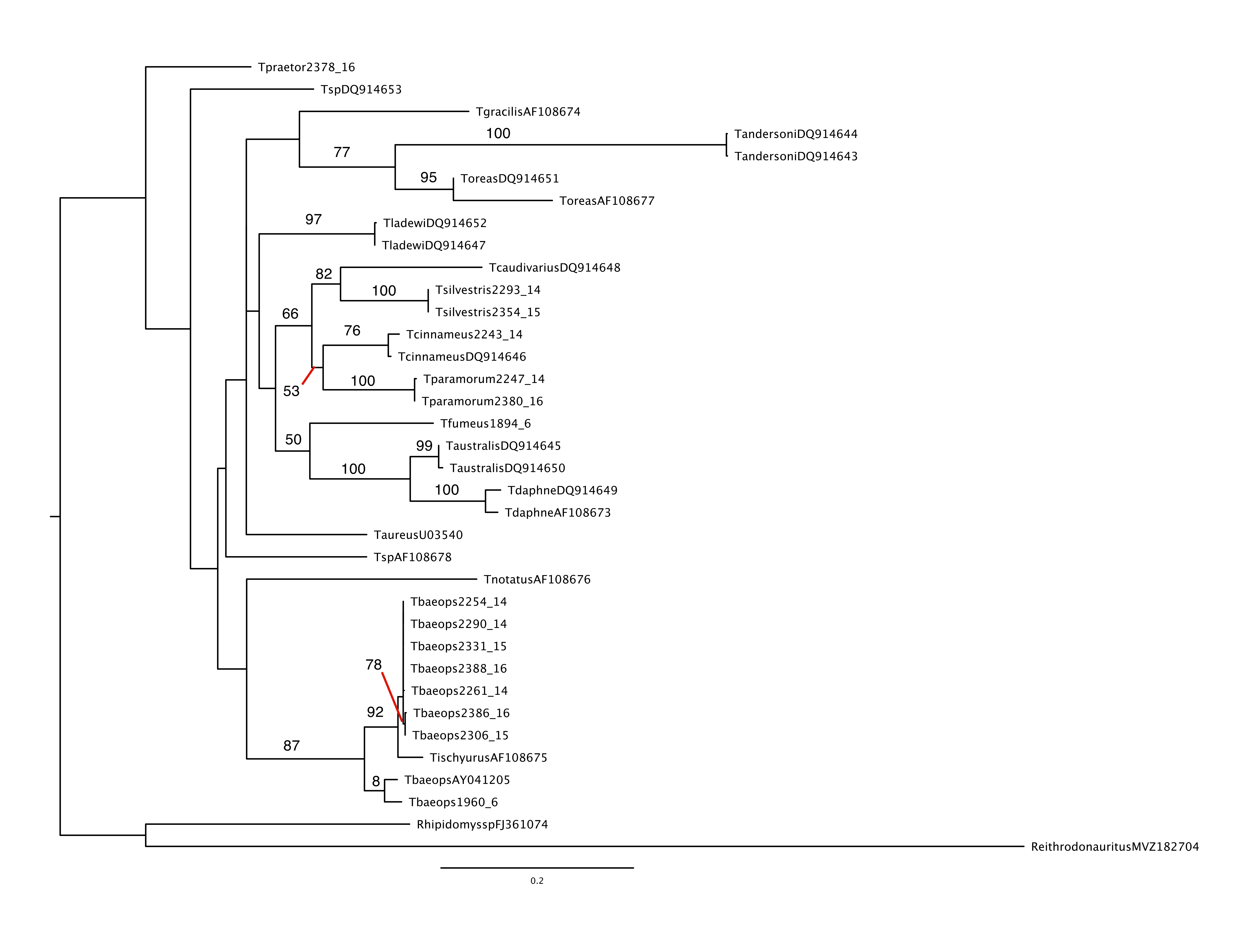
After Dr. Brokaw double checked the editing, we were ready to export the sequences into the Se-Al program. We used this program to line up the DNA sequences from different species to compare their differences and allowed us to see the actual amino acid sequences translated from the DNA for the rodent species. With this data we were ready to start conducting phylogenetic analysis of the rodents. We put the sequences into text format and used a command line program called PAUP to read the data and construct a quick bootstrap tree. The quick bootstrap compares the sequences by similarity of the bases and makes a tree showing the similar species grouped together on branches and gives a percentage for the confidence in each of the branches. These trees give you a quick picture, but they cannot be trusted for accuracy. We looked over the other tree types we could construct and ran a parsimony analysis; parsimony finds the tree that groups species in the way the requires the lowest number of mutations in order for all of the species on the tree to have started with a single DNA sequence in a common ancestor. The analysis type that we worked up to was a maximum likelihood tree which calculates the mutation rates for each of the bases and compares all the possible trees to come up with the most likely tree based on the likelihoods of the different types of mutations. Our maximum likelihood tree constructed with our edited sequence data is shown below.
During the process of making these trees we learned that the cytochrome b gene from mitochondrial DNA was notorious for having large amounts of homoplasy. One form of homoplasy is when bases mutate and then mutate back at a later time; if that happens then you are unable to account for the mutation with the sequence data. Another form is when different species develop the same kind of mutation but the mutations are not related by ancestry (convergent evolution). Needless to say, this is not a good thing when constructing a phylogenetic tree based on mutations. Even though our ML tree is the best estimate of the relationships that we can make, many of the branches in our tree image do not have bootstrap support numbers on them because there was little certainty that they represent the true relationships between species. Due to this susceptibility to homoplasy, Dr. Brokaw and I are exploring the RAG1 gene (from nuclear DNA) and conducting a new set of PCRs in hope that the data from this new gene will either confirm or help correct our previous findings.

