The Last Blog… A Reflection of a Tall Grass Prairie

This has been quite a year for me and Samantha, and our research with Dr. Brokaw.  We have learned a lot, about our research area in Oklahoma, about the ACU Biology Department (that has so graciously welcomed a couple crazy Ag majors tag along on their conference trips, Biology club meetings, and so on), and about how the research process works. It’s been fun! And this is the last blog I believe I’ll be posting, which is bittersweet. I’m thankful to Pursuit, to ACU, to Dr. Brokaw, and most of all, my awesome partner, Samantha, for this entire process.

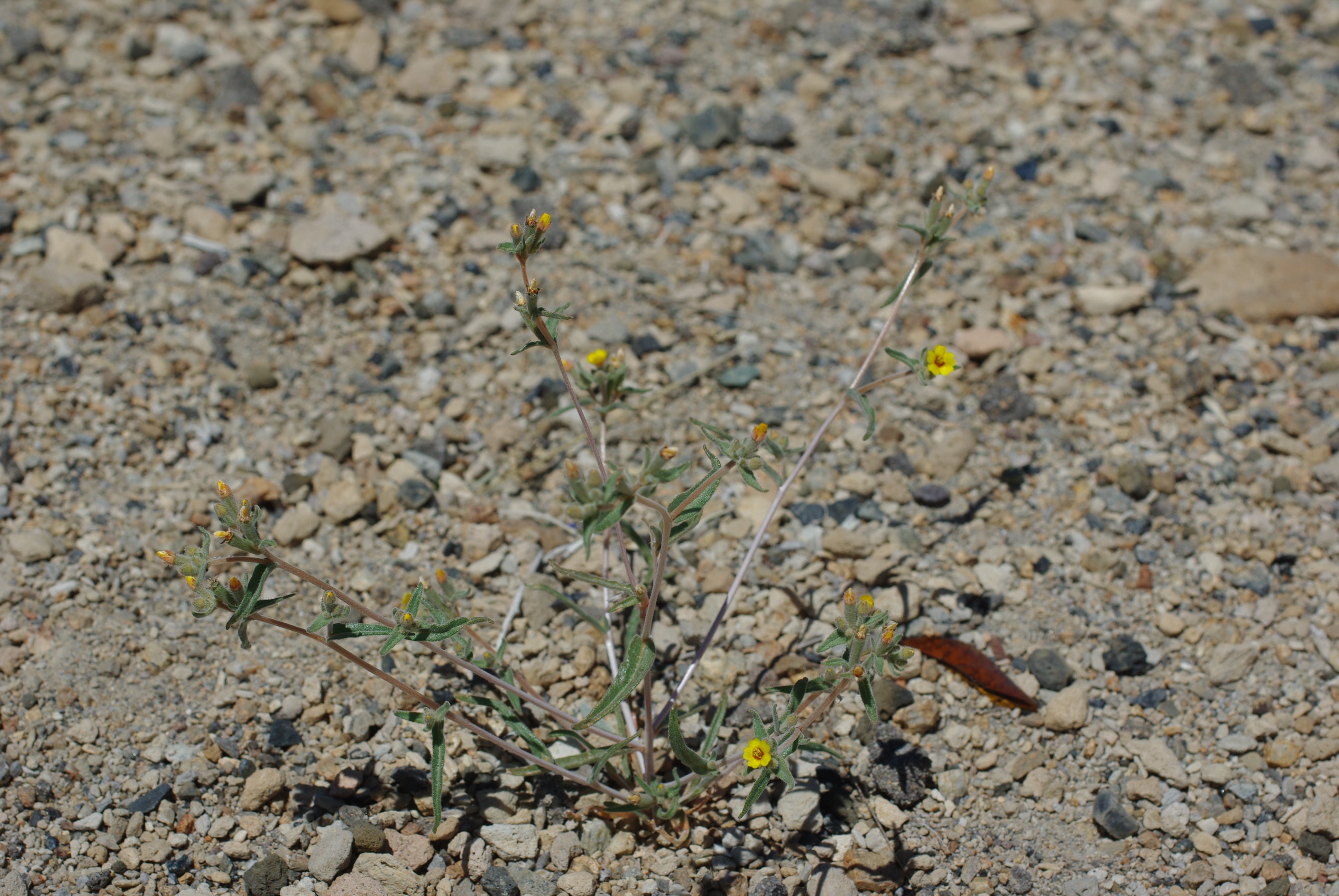
So far, our results have been as expected: disturbance-loving plants took over the spill sites, and the less competitive species have been in areas of lower hydrocarbon concentrations and on our control sites. In my opinion, we reached our goals as best as we could – seeing as how our goals were mostly to get through the samples at least one time this year (there were 40+ samples that we were trying to get through, on top of being full time students with jobs and families).

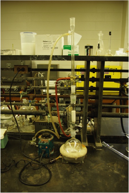
We smoothed out so many bumps in the road that will make way for the future: figuring out the fussy gas chromatograph, thinking we lost all of the research when I lost the thumb drive (it was mostly backed up, thankfully) and how to prevent that from happening again, coming up with a rhythm, and making decisions and alterations on so many little things that I can’t even remember them all now. Having these experiences, both traumatic and exciting, and getting through them successfully has encouraged me and enhanced my problem solving abilities. The extra activities I’ve gotten to participate in, like going to Hawley Middle School and talking to the kids for two years now, has helped me understand the importance of my research and how valuable it is to pass on the information and the interest of bioremediation. This alone has been an unexpected and pleasant surprise.Emily Adams Earth Day

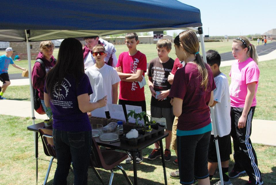
I am excited for the future of this project. I think a research endeavor like this, one that is about remediating an area that has been contaminated by a man-made accident, is really important for ACU and a great opportunity for its students. I will continue to work on this project for the next month or so, and hopefully in the fall I will be able to help with training another student to take over, since Samantha and I have graduated. I hope that the student is able to devote a lot of time to this, perhaps by securing their own grant, and are therefore able to work less (if at all) somewhere else; this is the only suggestion for change that I have – just having students that are available to spend a lot of time on the project. It’s the best way to keep consistency within the methodology of the project, and when it has worked best for us.Emily Adams Presentation

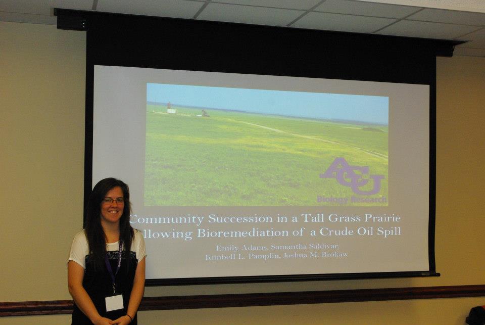
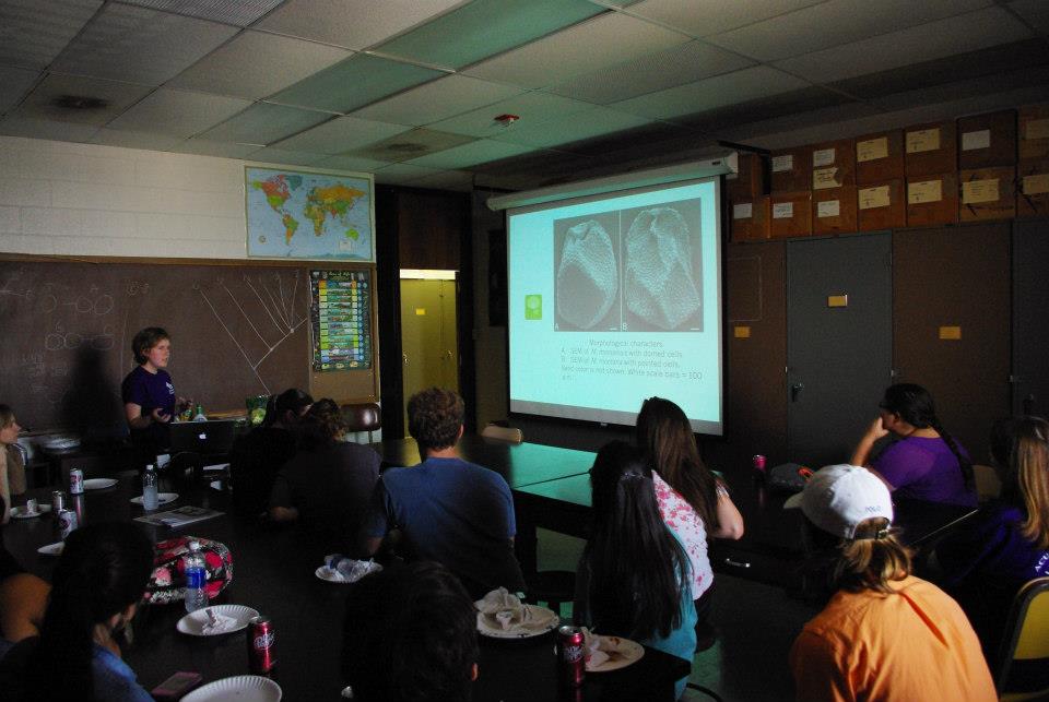
Bioremediation of a Tall Grass Prairie has been a great scholarly journey for me. Samantha and I have presented research at the ACU Undergraduate Research Festival and the Texas Academy of Science.  Both were great opportunities and I learned a lot about what I do well and what I don’t. I hope that this research project and what it taught me will be a solid foundation for the research I hope to get to do in the future.

Posted in Brokaw Lab | Tagged , , | Leave a comment

Mentzelia monoensis

Over the past several weeks, I have gradually been immersed into a whole new world: research. Often, it was intimidating; I found myself in positions of uncertainty and insecurity. I messed up a lot, which was humbling. But more importantly, I learned a lot. Research, I realized, is a learning process. Mistakes and frustrations don’t define the experience, rather our responses to these stressors do.Tina Presentation

What exactly have I been researching?  My research pertains to a plant known as Mentzelia monoensis, an allopolyploid endemic to Mono Co., California. While I won’t go into extensive detail (that’s what the introduction is for!), many difficulties arise in identifying the species from its relatives (due primarily to overlapping morphological characteristics). As the species’ true distribution is presently unknown, it is important to develop effective mechanisms to facilitate identification. Currently, we are planning on utilizing DNA barcoding, a method that utilizes short genetic markers to identify unknown specimen.  Below I have included the beginning of the introduction that I am writing for a paper that we would like to publish about this research.

My partial introduction, as posted, reflects part of this learning process. Often when I write, I want to use big words, words that procure (see, words like procure) the greatest effect. However, I discovered that flowery language can often confuse readers, especially in papers that already address difficult concepts. In writing scientific papers especially, message supersedes style. Clear communication is key. Likewise, there is no harm in having other professionals aid you in the writing process. Sometimes this can reveal weaknesses in your writing that you don’t notice.

Additionally, expertise is not a precursor to conducting research. This might sound a bit obvious, however perspective has a funny way of affecting thinking. Prior to researching, I felt that I had to be a walking textbook—I had to memorize and regurgitate all of the information I was given. But I soon discovered that memorization, though a useful skill, does not compensate for understanding. I could memorize all the steps in gel electrophoresis, but I didn’t understand the process until I actually performed one myself. Moreover, you don’t have to be an “expert” in the field you’re in researching in, especially initially. I will be the first to admit that I’m a novice when comes it comes to plants (especially compared to Dr. Brokaw). But that’s okay; I don’t have to be an expert (and I am certainly not expected to be).

My advice: try it. You never truly know how much (or how little) you’ll enjoy something until you experience it yourself. You might doubt your own abilities or feel intimidated by the new situations, but don’t let your fears impede the opportunities God places in your life. Rather, embrace what is given to you and share your abilities with the world.

Introduction:

Mentzelia section Trachphytum is a monophyletic group comprised of roughly 20-30 annual species in western North America, particularly in California (Darlington 1934; Zavortink 1966; Hufford et al. 2003; Brokaw and Hufford  2010a, b).  Trachyphytum is unique among sections of Mentzelia for its high number (approximately 2/3 of the named taxa) of polyploid species (Zavortink 1965).  The section is generally composed of species that either tolerate extreme soil conditions or colonize disturbed sites.  Mentzelia monoensis, is a recently described hexaploid species that lives in course pumice soils and disturbed sites of Mono Co., California (Zavortink 1965; Brokaw and Hufford, 2011).  This species is of particular interest because of its unique allopolyploid origin (Brokaw and Hufford, 2010b).  Mentzelia monoensis is the only allopolyploid within Trachphytum formed through a hybridization involving the two predominant clades, “Affines” and “Trachphyta” (Brokaw and Hufford, 2010b).

Recently, some experts have considered elevating M. monoensis to threatened status, and the California Native Plant Society currently ranks M. monoensis as a 4 (Plants of Limited Distribution), which indicates the species could potentially be vulnerable to environmental change (http://www.rareplants.cnps.org/detail/3657.html).  From collected data, the species appears to be narrowly distributed near Mono Lake and has only been observed in Mono Co., California (Brokaw and Hufford, 2011). The Mono Lake region itself has piqued the interest of conservationists as a result of unnatural diversion of water pathways to Southern California, resulting in extreme environmental change and, potentially, species endangerment (citation).  However, our current knowledge of the distribution of M. monoensis is only tentative.  This deficiency stems from both the short amount of time that M. monoensis has existed as a described taxon and, more markedly, the difficulty in distinguishing the species from others in Trachphytum (Brokaw and Hufford, 2011).

Morphologically, M. monoensis closely resembles other species in Trachyphytum, especially M. montana and M. albicaulis. Upon close inspection, one can usually identify M. monoensis based on knowledge of seed coats, floral bracts, and leaf color (Brokaw and Hufford, 2011).  However, identification can be time consuming and cumbersome, especially among those unfamiliar with Mentzelia. Furthermore, these characters are not available in all developmental stages. Morphological similarities between M. monoensis and its relatives can be attributed to two primary factors: allopolyploidy and time. First, most polyploid species in Trachyphytum are allopolyploids, which in turn leads to overlapping morphological variation in the section (Brokaw and Hufford, 2010b). Second, M. monoensis is a recently formed polyploid, meaning that it may not have had adequate time to develop unique morphological traits.  Consequently, M. monoensis—because of its recent speciationcannot be reliably distinguished from its progenitors, including M. montana (Brokaw and Hufford, 2011).

Posted in Brokaw Lab | Tagged , , , , | Leave a comment

Update on Mentzelia thompsonii

So, it’s been a while since I’ve posted on here. I am sorry for that. Alright, so last time I left all of you, Dr. Brokaw and I were still trying to figure out how to work the ArcGIS program to map out our climate data along with our current niche model for M. thompsonii. However, since then, we have given up. Dr. Brokaw introduced me to a new program called DIVA-GIS. This program even came with an easy to follow instruction manual that allowed us to finally make progress. With DIVA, MAXENT, and our climate data, we were able to create two different maps:

Map of locations that currently have climates suitable for Mentzelia thompsonii. Small green circles in western Colorado and eastern Utah represent current populations.

Map of locations estimated to have had climates suitable for Mentzelia thompsonii during the last glacial maximum.

These maps are only based on climate data, however, and show areas on the current possible distribution map where M. thompsonii has not been known to live. This means that we have to go into more detail with our map and introduce more variables to be more specific.

For our next project, Dr. Brokaw and I are going to introduce soil types and climate data into MAXENT and DIVA to create new maps of past, current, and future possible locations of M. thompsonii.

I will try and do a better job at keeping everyone updated as more work gets done!

Posted in Brokaw Lab | Tagged , , , , , | Leave a comment

That moment when….

This has been quite a semester for this project. It’s been a relatively discouraging process; I have often felt as though I wasn’t getting anywhere.

Yeah, I supposedly know how to use a gas chromatograph. Yeah, I know what the little lines given to me by the mass spectrometer mean. I’ve tutored [read: dragged] enough fellow classmates through Organic Chem lab write-ups and practicals that I could teach anybody how to use those machines. I could even teach you how to change the fiber glass wool filter … thingy. (It’s important.)

But that doesn’t mean when I put a tiny vial of a ~mL of concentrated hydrocarbons into the slots of a gas chromatograph, and the syringe descends into it, atomizing a tiny amount of the solution, sending it through a copper coil and through the many different sensors, that it will feel like it worked…

That doesn’t mean that I’m going to be confident that what I call results are, in fact, results. I’m probably going to sit and look at them for a while. After feeling okay enough about them and that I have gotten the information I needed from all the little peaks, I’ll probably look at it compared to the concentrations other people have found in the days of research past and feel like I messed something up.

On one of those days, when we were comparing my results to the control results we were using from a previous student’s research for this project (let’s call him Sam), Dr. B was expressing his concern that 1. our concentrations were a lot lower than expected, and 2. the graph we were using to determine the hydrocarbon concentrations in the sample was not accurate enough for our tastes at areas of low concentrations or at high concentrations. (That’s a problem.) Here’s Sam’s graph:


graph from former student's research.

The x-axis represents the concentration in milligrams of C36H74 per milliliter of cyclohexane (C6H12); the y-axis represents the total of peak areas. So, the blue dots along that curved line are the measured peak areas of hexatriacontane (C36H74) at each concentration. These numbers are supposed to give us sort of a control in our project. That Y= equation at the top is supposed to be what we use to convert the numbers we get from the runs that I do from the oil spill samples to actual hydrocarbon concentrations in the soil.

But, that curve is a bad thing. When trying to represent the relationships of concentration ratios, a straight line is what’s desirable… By “desirable,” I mean that if your line isn’t straight, something is wrong. Either your technique is poor or your machine isn’t working well. In this case, it turns out to be a bit of both. At the top, where the line curves, it seems that the concentrations used were so high that they were breaching the detection limits of our GC… So we removed the high numbers from the graph, and it looked a little better.

When we would take the total peak areas of hydrocarbons from our soil samples and plot them, our numbers were coming in at the bottom of that line (at the low concentration levels), but not exactly in line with Sam’s numbers. (Our guess is that the concentration levels were so low — less than 1 mg C36H74 per mL of C6H12 — that he was unable to measure the tiny amounts of C36H74 accurately.) So we decided that we would start from scratch, and I would run all new concentration controls.

So I did that, and this is the graph we got:

Hooray! Our line is straight! R2=1! (That’s a good thing!) This is a graph that plots all of the control samples I ran, plus two measurements from Sam that we felt were accurate (the two highest concentrations in this new graph). And it works! Now we have an equation we can use and feel good about it.

You know that moment when you finally feel like you did something right? When you finally feel like you know what you’re looking at? That you know you can move forward with confidence?

Success in science is a good feeling. Even at (or perhaps, when it comes to undergraduate research, especially at) the most basic levels.

Posted in Brokaw Lab | Tagged , , | Leave a comment

Thomasomys Phylogeny Continued

In early October we received our sequence data back from the Yale DNA Analysis Facility. The sequence data gave us both the forward and reverse strands that we copied using PCR for each of our rodent species. We had two samples with either shortened or ruined sequence data for one strand that we could not use, but even so we had one sequence with a decent enough result that we could read the whole length from the one strand that worked. The next step that we took was to pull the sequence data up in a sequence editing program and arrange the sequences into “contigs”; this means we paired the sequences into groups of forward and reverse strands so that we could edit the sequences. We have to edit the sequences because the machine can make mistakes and make the wrong call on certain bases where it has overlapping base signals or weak data. We edited the sequences by first comparing the forward and reverse strands for individual samples to see if the strands matched; the purpose for having both strands is so that there will be overlap that can be used for comparison. Sequence data is often weaker and less reliable farther down the strand from its given primer so having the other side allows for clearer data at the extreme ends. As we got farther into the editing we compared larger groups of samples together so that we could see the similarities and make sure we made consistent ‘calls’ during the editing process.

DNA Data in a Sequence Editing Program

After Dr. Brokaw double checked the editing, we were ready to export the sequences into the Se-Al program. We used this program to line up the DNA sequences from different species to compare their differences and allowed us to see the actual amino acid sequences translated from the DNA for the rodent species. With this data we were ready to start conducting phylogenetic analysis of the rodents. We put the sequences into text format and used a command line program called PAUP to read the data and construct a quick bootstrap tree. The quick bootstrap compares the sequences by similarity of the bases and makes a tree showing the similar species grouped together on branches and gives a percentage for the confidence in each of the branches. These trees give you a quick picture, but they cannot be trusted for accuracy. We looked over the other tree types we could construct and ran a parsimony analysis; parsimony finds the tree that groups species in the way the requires the lowest number of mutations in order for all of the species on the tree to have started with a single DNA sequence in a common ancestor. The analysis type that we worked up to was a maximum likelihood tree which calculates the mutation rates for each of the bases and compares all the possible trees to come up with the most likely tree based on the likelihoods of the different types of mutations. Our maximum likelihood tree constructed with our edited sequence data is shown below.

Maximum Likelihood Tree for Thomasomys Samples


During the process of making these trees we learned that the cytochrome b gene from mitochondrial DNA was notorious for having large amounts of homoplasy. One form of homoplasy is when bases mutate and then mutate back at a later time; if that happens then you are unable to account for the mutation with the sequence data. Another form is when different species develop the same kind of mutation but the mutations are not related by ancestry (convergent evolution). Needless to say, this is not a good thing when constructing a phylogenetic tree based on mutations. Even though our ML tree is the best estimate of the relationships that we can make, many of the branches in our tree image do not have bootstrap support numbers on them because there was little certainty that they represent the true relationships between species. Due to this susceptibility to homoplasy, Dr. Brokaw and I are exploring the RAG1 gene (from nuclear DNA) and conducting a new set of PCRs in hope that the data from this new gene will either confirm or help correct our previous findings.

Posted in Brokaw Lab, Lee Lab | Tagged , , , , | Leave a comment

Faith and Trust

While setting up my samples to run overnight in the lab I am always fearful. What if I did something wrong? What if this thing falls over (It’s pretty tall)?

Soxlet Extraction Apparatus

Soxlet Extraction Apparatus

What if the cyclohexane evaporates and the heating mantle causes the boiling flasks to break? What if housekeeping turns the water off to my experiment? What if the room temperature changes and I have the heating mantle set too high/low to account for the change (we all know FSB has the craziest heating/ cooling system ever.) As I lock the door to leave I often feel like a parent (yeah I know soil is my child…my labor of love..yadda yadda) last night especially. I had this sinking feeling that something was going to go wrong, so I said a little prayer and had faith that I had set everything up properly. No matter how much experience I get at the set, up I always feel this way; my first child is leaving for their first sleepover and I am worried “Ok little soil sample, be good, play nicely with the cyclohexane and I do not want to get a call from the parents saying you blew something up.” Faith and Trust.

Trust that the experiment is sound, that FSB will not have some crazy thermostat problem in the night, that the housekeeping people will leave my stuff alone….Trust.

Faith….faith that there are hydrocarbons in my little baby soil sample and that all of this wasn’t for nothing. Faith in the GCMS (yes faith, if you have ever used it you know its an act of God if it is working reliably).

I know you won’t want to hear this, because the people who do undergrad research are often those same people who hate group work…but learn to work in a group..with a partner…I have had my fair share of HORRIBLE partners, and it was nice to get that out of the way before I hit the “Real World.” If I hadn’t gotten used to group projects before, I would have a hard time working with even the best of partners (which for the record mine is :).

Oh yeah, and when your partner loses your data (and you think for a split second before you get your bearings that you might punch her) remember that everyone makes mistakes. Most mistakes are fixable–and I know I have made my share. So Emily- I would rather hug you than hit you..which I will do.

Posted in Brokaw Lab | Tagged , , | Leave a comment

Mentzelia thompsonii

Hey everyone,

Populations of Mentzelia thompsonii sampled from western Colorado, northwestern New Mexico and eastern Utah. Stars represent sample locations. Colors of stars represents different DNA types (haplotypes). Stars with different fill and outline colors represent populations with two haplotypes.

So, this post has been very belated! My name is Jonathan Stites and I am currently a junior biochemistry major (ministry minor) at ACU. I conduct biogeography/phylogenetic research under Dr. Brokaw.

Basically, what this research entailed, was collecting specimens of Mentzelia thompsonii and extracting their DNA. From there, we then compared the nucleotide sequences of the specimens to find the mutations within their chloroplast DNA. The number of mutations that we found demonstrated how far apart these plants are from one another in a phylogenetic tree. Attached is the poster that Liz Lurz and I presented at the ACU undergraduate research festival.

Lurz-Stites et al. Poster

Currently, I am using arcGIS and MAXENT software to incorporate the data from above (and in the poster), climate data, and soil types to predict where these plants may be in the future. Updates to come!

Posted in Brokaw Lab | Tagged , , , , | Leave a comment

Rodent Phylogeny Progress

This month we made a huge step toward our short term goal of sending off the Thomasomys DNA samples for sequencing. Dr. Brokaw and I found a set of primers that could amplify an approximately 1200 base pair region of the cytochrome-b gene that we are working with. We tried several primer sets and had to run a large number of PCRs in order to determine which primer set gave us the best amplification results with the largest number of our rodent DNA samples. One step in our progression towards determining the best method for amplification was running a gradient PCR to try the reaction at various temperatures (the same DNA sample is run at a number of different annealing temperatures), through this we learned that a slightly lower annealing temperature (46° C) than our previously used temperatures (50-54° C) gave us the best results.

Gel of gradient PCR performed on a single DNA source amplified using the p484-p485 primer pair. Annealing temperatures from left to right were 44.5, 46.2, 48.1, 50.0, 51.9, 53.8, and 55.7 degrees Celsius.

However, we hit quite a snag in our research when our PCR reactions inexplicably stopped working; we were using the same primers, samples, reagents, and PCR profile as a previously successful experiment. The last few weeks of summer and the first of the semester Dr. Brokaw and I had to backtrack in order to identify what element was hindering our progress. We systematically ran PCRs substituting out various reagents and ingredients of our experiments. After a number of consistent failures, we remixed our primers and revisited a procedure that had worked previously, to our relief we found bands in the gel once more (in the right base pair region to boot).  We still aren’t sure, but it is possible that poor water quality was the problem.

Sep 3,2012 gel (remixed primers)

Gel of 15 DNA samples amplified with the remixed p484-p485 primers.

After moving past the hiccup in our research, I used the newly mixed primers (with good water) and ran another PCR with a gradient to try and get all the samples to show adequate amplification. With good results on the PCR, we preformed a cleaning using a Cycle Pure kit. Tanya and I quantified the DNA from our cleaned samples using a NanoDrop to make sure we retained our DNA and had adequate amounts. We will be sending off the samples to be sequenced later this week. When they return, our next step will be to start the DNA editing for the phylogenetic study.

We are also in the process of a DNA extraction from liver tissue to prepare new samples provided by Dr. Lee and his research assistants. The data should be quite interesting to compare with our previous samples as they were collected on opposite slopes of the Andes mountains.

Posted in Brokaw Lab, Lee Lab | Tagged , , | Leave a comment

Back to a routine….maybe

During the first week of school Dr. Brokaw taught me how to use the computer program that I will need to do the Detrended Correspondence Analysis (DCA) of our Tallgrass Prairie vegetation plots. The program is called Canoco. It is not the kind of program you could just use common sense to muddle through, and I am sure that knowing how to use it will be useful in the future. I completed my first analysis on my own later in the week, but I need to have my work checked before I am confident that I got everything done correctly. I have included an example DCA from last year.  We use DCA to show how similar the vegetation types on each of our plots are; sites that are similar will be close together on the DCA diagram.

Detrended Correspondence Analysis From 2011 Vegetation Data. Red squares represent species composition of spill site quadrats. Green circles represent tilled control quadrats. Blue triangles represent native preserve sites.

Dr. Brokaw, Emily and I met to go over what we expect from this year and a time frame for accomplishing our goals……all dependent on the GCMS (gas chromatography–mass spectrometry) working properly. Last year the GCMS was continually either broken or being used, and we failed to gather much data because of that set back. We were crossing our fingers that this year would not be the same but we are already off to a bad start.

Emily went to go run a sample from last year just to be sure that we could get results using the GCMS before I take off on running all the samples through the cyclohexane to avoid wasting our resources. Unfortunately, the GCMS is out of helium…..again….which means that we are already behind schedule. [Editorial note from Dr. Brokaw: But hey, no one is complaining here!]

Our plan called for some wiggle room so I hope we can get on track soon.

Posted in Brokaw Lab | Tagged , | Leave a comment

August Microbiology Research

The month of August tested my ability to not only accomplish my own work, but to perform the tasks of my two research partners while they were away on vacation. The key words for the summation of my success were organization and documentation.

I began the month where I left off in July, with the attempt to perform a gel DNA recovery on tapY1. All I can say is frustration. Every time I performed this process with the appropriate kit, I received poor results on the Nanodrop (I was hoping to receive a nucleic acid concentration of at least 200ng/ul, but the highest I obtained was 50.0ng/ul). The gene sequence, recA, was also ready for gel DNA recovery, and to my dismay, the results displayed extremely low concentrations. Both tapY1 and recA were sent back to the stage of large-scale PCR using AccuTaq. The gene sequence, clpAS, finally reached the stage of moving from PCRs with Taq to PCRs with AccuTaq. First, I ran an AccuTaq PCR gradient to discover the proper annealing temperature. Second, I ran a large-scale AccuTaq PCR using the appropriate annealing temperature to amplify the 4.6kb product. Once the large-scale PCRs for tapY1, recA, and clpAS were all run, gel DNA recovery was attempted one final time.

Yikes! Not only were the results extremely poor, but also, the gel run with the DNA recovered products produced fuzzy bands, all of which were the wrong size. Just when I started thinking progresses was being made, I learned that backtracking was the new trend of my research. I set up Nesting PCRs for tapY1, recA, and clpAS using their innermost primers and the gel recovered DNA as the template DNA. This protocol was used to confirm whether or not the recovered DNA came from the appropriate section of the genome. Thankfully, the correct band sizes were produced! I proceeded to large-scale PCR for tapY1, recA, and clpAS using the outermost primers and the gel recovered DNA. The gene sequence, recA, was successfully amplified, but unfortunately, tapY1 and clpAS were not. The recA product was cleaned-up with a PCR Inhibitor Removal Kit and stored in the freezer until ready to send-off for sequencing. Finally, I advanced tapY1 and clpAS to the stage where their products were able to be cleaned-up with the PCR Inhibitor Removal Kit.

Gel with SYBR Green

Gel with Ethidium Bromide

When the gel was run with all the PCR purified products, tapY1 and recA both displayed multiple bands. Also, the bands were not tight, but very wavy. A serious decision was made to transition from using SYBR green gels to using ethidium bromide gels. Although the health risks are higher from ethidium bromide, the gel bands are much tighter, without drags. Finally, the day arrived when all of the DNA samples were ready to be sent off for sequencing. I diluted the PCR purified products for tapY1, recA, and clpAS, and I diluted all of the primers for each of the three genome regions. Sufficient organization, color-coding, and packing were insured to make the parts to the puzzle easy for the sequencing company to distinguish. How exciting it was to reach this initial goal of research! When the results returned, the company concluded that almost all of the data was bad. Future research will consist of comparing the returned sequences with predicted Geneious results to determine whether the sequences are usable or not.

A side project I worked on this month was constructing a replica-plating device out of a plastic cup, ring clamp, foam board, and a Kleenex. My design was a success, but the Kleenex hypothesis was not a sufficient replacement for the original velvet. The texture of the Kleenex was to thin and absorbed the media liquid, effecting the bacteria’s transfer onto a new TSA plate. Test will be run in the future to determine whether velvet will work on my device and allow adequate replica-plating. A huge discovery this month was that the deionized water in the microbiology lab and the research lab registered a pH of 1.9, instead of 7. Oh, no! No wonder so many test resulted in poor results! The acidity was killing the microorganisms. At least the mystery has been solved, and research can continue with a new sense of awareness of how important the pH of water really is! Summer research has been an exciting and rewarding experience. Now that school has begun, a new challenge I face is scheduling time to continue my research. I am excited to see how my research will progress during the month of September.

Posted in Huddleston Lab | Tagged , , , | Leave a comment